Exercise 2-2 Specification of unit model parameters.
In this exercise you will use the job that you started in exercise 2-1. If this is not your current job, close the current job and open the job you previously saved in exercise 2-1.
Edit the unit model parameters. (This can be accessed form the main Edit menu).
For this exercise you should use the Plitt hydrocyclone model which you will find described in Section 4.5.7 in the textbook or in Technical Notes 3. The model is identified as model CYCL in MODSIM.
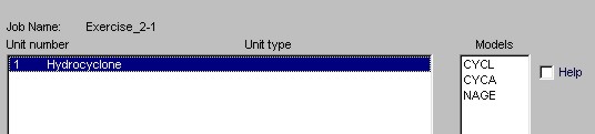
The flowsheet for this exercise includes only a single hydrocyclone so there is only one entry in the "Units" block of the "Select models and parameters for units" form. Click on "hydrocyclone" and the models that are available for a hydrocyclone will be listed in the "Models" list. Note MODSIM uses 4-character mnemonics to identify unit models. Check the "Help" box if you wish to see a brief description of the model before you specify the parameters. Double click on the model that you wish to use. If "Help" is checked you will see a description of the model including a description of the parameters that are required for the model. At this stage you can elect to accept the model or cancel your selection and try another model.
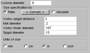
The forms that are provided to specify parameters for the unit models are unique and each model has its own form. Some are very simple and some are quite lengthy including more than 20 parameters for complex models such as those for autogenous mills. The form for specifying parameters for the Plitt hydrocyclone model looks like this.

For this exercise use the default values for all parameters except the cyclone diameter. Choose a cyclone of 60 cm diameter with standard geometry. Accept this data and click Accept and you are back on the "Select models and parameters for unit" form. Click accept to accept all parameter model parameter data for this flowsheet.
Save the job.
Open the main Run menu and click "Run simulation". If you do not get the "Simulation was completed successfully" and the "Data output completed successfully" messages you have specified some data badly. Review your system data and model parameters carefully.
It is unlikely that anything will go seriously wrong in this simple exercise so you should be able to see the results of the simulation now. This is a good time to save the job.
Open the main View menu and view
the flowsheet. The flowsheet appears and you can get an immediate
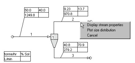
summary of the plant behavior from the data in the stream flyouts.

Note in particular that the overflow has 13.7% solids and the underflow 70.9% solids. (If you do not see these values you have not specified some of the data as required and you ought to check all your data before proceeding. If you cannot find any error you should get job Exercise 2-1 from the Internet. (If you have not used this feature before, watch the viewlet "Loading a JOB from the Internet" in the MODSIM Trainer). The 70.9% solids in the underflow should catch your attention because a hydrocyclone will probably rope when discharging such a dense slurry. This will be discussed further later in this exercise.
The first thing to note are the units that are used to display the flowrates in the flyouts. The defaults (kg/s) should be showing in this exercise. In most problems you will want to choose more appropriate units. To do this you must leave the flowsheet (Select Accept flowsheet or Cancel from the File menu) and edit the output format. (Open the main Edit menu and choose "Edit output format"). Select tonnes/hr in the "Units for solid flowrate" block and L/min in the "Units for water flowrate" block. Uncheck the "Display latest output data" box and click "Accept". View the flowsheet again. Note that the flyouts now display quantities using the units that you have selected. The lower right space in the flyouts is reserved for the display of metal content. This will be covered in a later exercise.
You can obtain more information about the properties and composition of any stream by right clicking on the stream while viewing the flowsheet. This will pop up a menu from which you can select the "Stream properties".
|
Right click on a stream to see its properties |
This will display most if not all of the information that you may wish to obtain about the stream including flowrates, solid yield and the particle size distribution in the stream. The d80, d50 and d20 sizes of the solids are also given. Right click on the overflow stream and note that the d80 size for the cyclone overflow is 81.6 microns. Right click on the underflow stream and note that the d80 size for the underflow is 516 microns.
You can also display a plot of the particle size distribution in the stream.
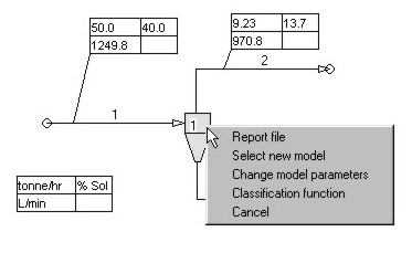
The next type of data to look at is the report on the operation of the hydrocyclone. This is contained in the report file for the unit which is produced whenever the simulation is run. The easiest way to access the report file for the unit is to right click on the unit icon for the hydrocyclone and select "Report file" from the pop-up menu.
|
Right click on the unit to see its performance. |
A formated file is displayed that is specific to the simulated performance of the unit. Scroll through this file and note the kind of information that is displayed. In particular note the following items: the parameters used are shown for reference, the size distributions in the feed and product streams are tabulated and the calculated d50c size for the operating conditions (90.9 mm) is shown. The actual d50 achieved can be read from the graph of the actual classification function which can be displayed by selecting the "Classification function" item from the pop-up menu Note that at the bottom of the file a warning is issued to the effect that the Mular-Judd criterion indicates that the cyclone will rope in operation. This correlation suggests that a spigot diameter of at least 7.4 cm is required to prevent roping. Furthermore the Concha analysis indicates that the air core diameter is 13% larger than the spigot diameter. This also indicates that roping can be expected. Before proceeding it is advisable to fix this potential problem. Recall that a 60 cm diameter cyclone was chosen with "standard" geometry. This requires the spigot diameter to be 11.6% the cyclone diameter which is equivalent to 6.9 cm. So now go back to edit the unit parameters and set the spigot diameter to 15% of the cyclone diameter. This can be done most conveniently by selecting "Change model parameters" from the pop-up menu. The new data looks like this.
RUN THE SIMULATION AGAIN and view the flowsheet. This is done most easily by right clicking anywhere on the flowsheet background and clicking on the "run simulation" pop-up. You could also use the main menu bar or go back to the main Run menu. Notice that the underflow is now 55.1% solids. Look at the report file for the hydrocyclone and note that d50c is now 75.8 mm. At the bottom of the file you will note that the Mular-Judd criterion is still issuing a warning but the Concha formula indicates that operation is fine with an air core 92% of the spigot diameter. In our experience the Mular-Judd criterion is too conservative and flags a warning too easily. Although we always take note of a warning like this, it is always necessary to exercise some judgement about it. (A well substantiated criterion for cyclone roping would be a valuable addition to the cyclone model so please let us know if you have any good operating data which could be used to develop a better criterion). This is a good time to change the job name to Exercise2-2 and save the job.
The next type of output data that are of interest are the particle-size distribution graphs. These are accessed from the View menu by selecting "Size distribution graphs". This will display the "Plot size distributions" window. Double click each of the three streams and these will be placed in the graph list. Click View graph to see the graphs.
At this point you will probably want to see the difference in the overflow size distributions that resulted from the increase in spigot diameter. In order to do this, it is necessary to accumulate the size distributions from the separate simulations outside of MODSIM. (Remember that MODSIM handles only one job at a time). The most conveient way to save a size distribution is to right ckick on the stream in the flowsheet and select "Plot size distribution' from the pop-up menu. This shows a small graph of the size distribution of the material in the stream. Right click anywhere on the face of this graph and you will be able to save the size distribution as a comma delimited file which will import nicely into many other applications including an Excel spreadsheet. For our purposes the Graphics for Mineral Processors application is specially convenient. If you have not already done so this is a good time to install it from the course CD-ROM or download it from the course site and install it. Start Graphics for Mineral Processors (It usually shows up as a program named PSD - short for particle size dostributions- if you did not specify another name during installation) and select "Size distributions" from the select menu. Import the saved size distribution file( it has the file type .csv)
Run Exercise 2-1 again and save the size distribution of the overflow as described above. Import this into "Graphics for Mineral Processors" and select each distribution into the graph list by double clicking. Display the graph. (Log - log coordinate system is probably best but feel free to experiment). Look carefully and you will see that in spite of the smaller d50 size with the larger spigot the overflow size distribution is slightly coarser. Why? (You will need a sharp understanding of the behavior of hydrocyclones to answer this. Here's an incentive. There is a 2 point bonus for any for-credit student who can post an explanation on the bulletin board. A careful review of of Section 4.5.4 in the textbook or Technical Note 3 should supply the answer.)
That completes exercise 2-2. You may wish to vary some of the other parameters in the cyclone model now and check the results. In fact you could really spend some time and put the Plitt model through its paces. You can also experiment with the other models that are available for simulating hydrocyclone classifiers. You should now tackle exercise 2-3 from objective 1