Exercise 8-1 Assessment of a rod and ball mill circuit.

The data given in the spreadsheet resulted from a careful sampling campaign on an operating plant. The spreadsheet can be viewed by clicking here.

In particular, both feed and product streams were sampled for the rod and ball mills. These data were used to estimate the breakage and selection function parameters for both of these mills. In each case the average residence time of the solids in the mill was estimated from the mill dimensions, the media load and the estimated flowrate through the mill. The values found for the residence times were 3.40 minutes in the rod mill and 2.19 minutes in the ball mill. The simple perfectly mixed mill model MILL in MODSIM was used for the ball mill and the model RODM was used for the rod mill. The least-squares best estimates of the parameters are given in Tables 1 and 2. Since the size distrinbution in the cyclone feed was not measured during the sampling campaign, the parameters for the cyclone could not be estimated directly.

Table 1 Estimated parameters for the rod mill.

Selection function	Breakage function
S1 = 1.658 1/min	beta = 3.696
alpha = 0.602	gamma = 1.481
mu = 1.4 mm	delta = 0.0
Lambda = 0.736	Phi = 0.242

Table 2 Estimated parameters for the ball mill.

Selection function	Breakage function
S1 = 1.508 1/min	beta = 7.699
alpha = 1.662	gamma = 0.683
mu 1.4	delta = 0.0
Lambda = 0.735	Phi = 0.683

These values can be tested in the simulation and the calculated size distributions can be compared to those measured during the plant sampling campaign. The comparison is facilitated in MODSIM since the measured data can be entered as part of the system data. The measured data are entered using the system data form. Double click on each stream for which measured size distribution data are available and enter the experimental data in the usual way. It is a good idea to specify a name for the stream at the same time. The information that is entered in this way is not used by MODSIM for simulation calculations in any way. It is merely displayed in the graphs for comparison.

The physical dimensions of the hydrocyclones were specified in the data set and under normal opertaing conditions no other infromation is required to specify the operation of the hydrocyclones if the Plitt model is used. The feed head was estimated to be 3.81 m. However in practice the cyclones should be calibrated to match the actual operation. Three calibration factors are provided in the model for this purpose. It is a simple matter to adjust these using least-squares stimation to find a good fit to the experimental size distributions. In this case the factors found were for D50c, 0.293, for the sharpness index 0.152 and fo rthe flow split 0.856.

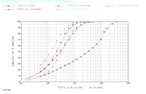
The resulting simulated output for this plant is shown in Figure 1.

Figure 1 Simulator output for the plant as sampled. Points are experimental data and lines are the simulator output.

It should be immediately obvious that the simulation is a good representation of the actual plant operation since the size distributions match the experimental data well. However, this is an example of a poorly operating milling circuit. Note how the rod mill is accounting for the greatest portion of the size reduction. The ball mill is not producing as much size reduction as it could if the circuit were set up more appropriately.

Some unusual aspects of this data are apparent. The media for the ball mill are described as slugs rather than balls. This means that the media are not spherical but have flat surfaces which have the effect of cushioning the very fine particles. This shows up as an unusually high value for alpha (1.662) in the selection function for the ball mill. This makes the specific rate of breakage fall off rapidly as the size deceases. This can be seen by inspecting the selection function for the ball mill. ( Right click the mill icon when viewing the flowsheet). In this case this leads to inefficient grinding in the ball mill.

Both the spigot and vortex finder diameters are unususally large in this plant. This gives rise to an unusually large cut point for the size of cyclone that is used.

You should now try to suggest changes that will improve the performance of this plant. Things you should consider are replacing the slug media with balls and using cyclones with a more conventional geometry. To simulate the effect of using balls rather than slugs you can simply change the value of alpha from 1.662 to 1.0 in the ball mill. The cyclones could be changed to the "standard" geometry (use MODSIM default values) and the three calibration factors to 1.0.

You should produce results that are similar to those shown in Figure 2 which represents a significantly better performance for this plant than the original data.

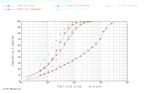
Figure 2. Size distributions under improved plant conditions. The data points represent the original plant operation and they are shown for reference.